The Lorenz attractor is based on a set of three equations (called the Lorenz equations) that describes the pseudo chaotic trajectory of a point in the 3D space. These equations have been found by Edward Norton Lorenz when he worked on complex weather simulations at the MIT.
The three equations are the following:
dx/dt = S (y - x)
dy/dt = x (R - z) - y
dz/dt = xy - Bz
where S, R and B are the system parameters (constants). These equations allow to compute the variation of the position for a small variation of time.
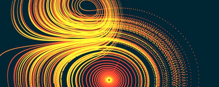
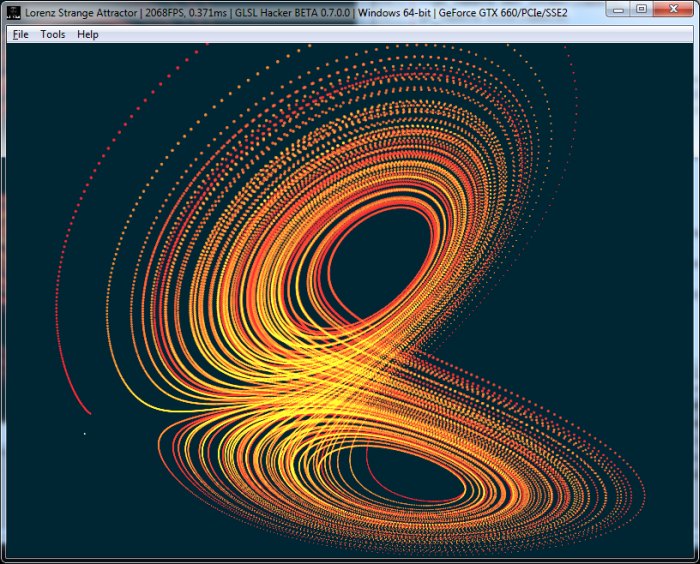
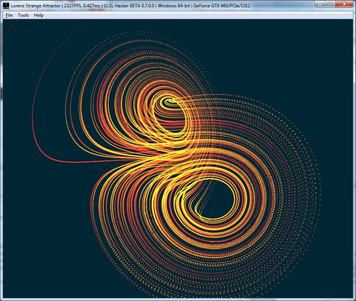
We get this well-known picture for a particular value of the three parameters (S=10, R=28 and B=8/3):
Lorenz attractor for S=10, R=28 and B=8/3
But other values produce similar shapes like {S=10, R=30, B=4} or {S=45, R=45, B=8/3}, see screenshots at the end of the article.
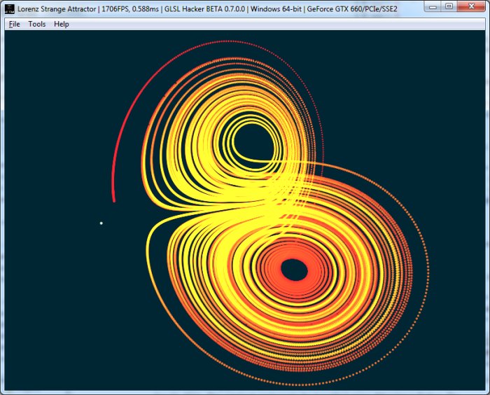
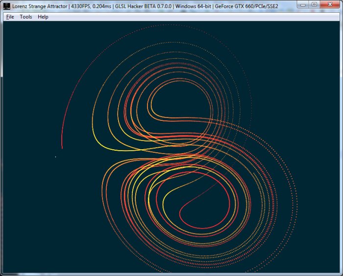
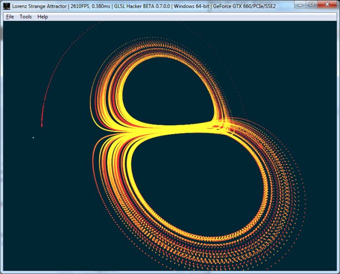
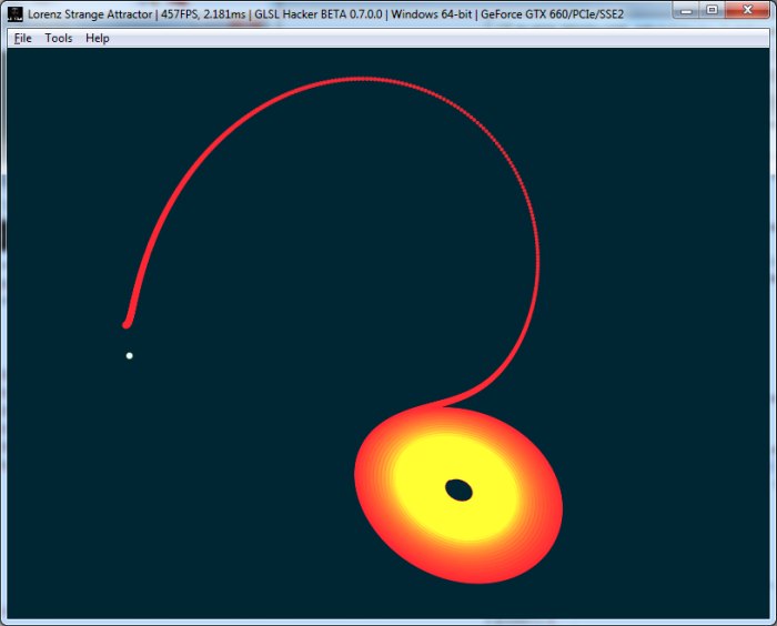
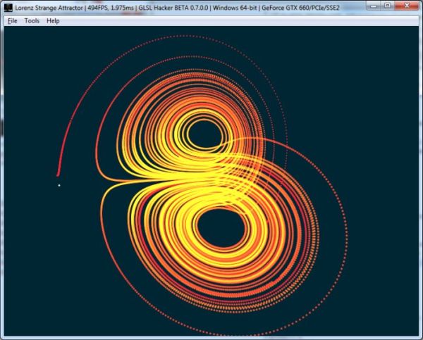
The Butterfly Effect: two initial positions with a very small difference (for example P0={x=2; y=2.02; z=2} and P1={x=2.01; y=2.03; z=2.01}) will produce two different trajectories. In the following screenshots, the difference between the initial positions is 0.01:
butterfly effect – P0={x=2; y=2.02; z=2} – S=10, R=28 and B=8/3
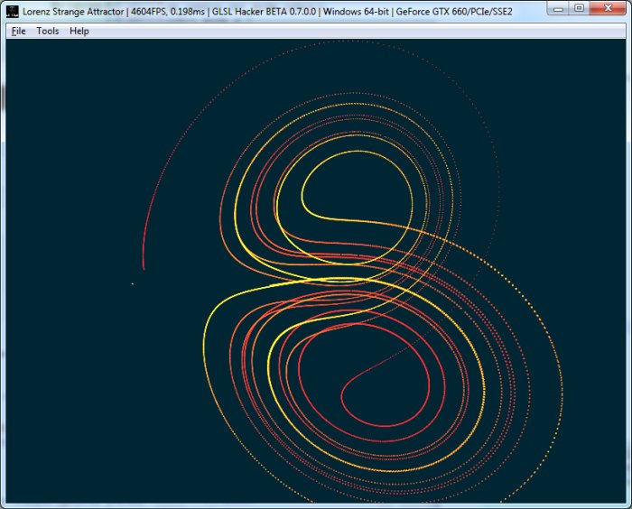
butterfly effect – P0={x=2.01; y=2.03; z=2.01} – S=10, R=28 and B=8/3
The name butterfly effect comes from the shape of the trajectory that looks like the wings of a butterfly. Here is an explanation of the bufferfly effect from wikipedia:
In chaos theory, the butterfly effect is the sensitive dependency on initial conditions in which a small change at one place in a deterministic nonlinear system can result in large differences in a later state. The name of the effect, coined by Edward Lorenz, is derived from the theoretical example of the details of a hurricane (exact time of formation, exact path taken) being influenced by minor perturbations equating to the flapping of the wings of a distant butterfly several weeks earlier. Lorenz discovered the effect when he observed that runs of his weather model with initial condition data that was rounded in a seemingly inconsequential manner would fail to reproduce the results of runs with the unrounded initial condition data. A very small change in initial conditions had created a significantly different outcome.
The wings of a butterfly
Here is a code snippet that shows how to plot a point P:
function InitPosition()
  P.x = random()
  P.y = random()
  P.z = random()
end

function UpdatePosition(dt)
  dx = 10 * (P.y - P.x) * dt
  dy = (P.x * (28 - P.z) - P.y) * dt
  dz = (P.x * P.y - 8/3 * P.z) * dt

  P.x = P.x + dx
  P.y = P.y + dy
  P.z = P.z + dz
end


InitPosition()
while(true)
  UpdatePosition(dt)
  DrawPoint(P)
end
I coded a small demo with GLSL Hacker that visualizes the path of a point following Lorenz equations. And to make the demo more compelling, each and every position is displayed, showing the full trajectory instead of a single point that moves from one position to the other one.
The demo (in Lua + GLSL) is available in the host_api/Particle_Lorenz_Attractor/ folder of GLSL Hacker demopack. The demo uses a vertex pool (an big array of vertices) to render the Lorenz attractor. To set the initial position, look at around line 81. To change the Lorenz equations parameters (S, R and B), jump to line 180.
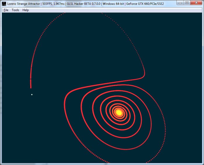
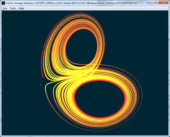
Here are some shapes of the Lorenz attractor for various values of S, R and B:
Lorenz attractor for S=45, R=45 and B=8/3
Lorenz attractor for S=60, R=28 and B=8/3
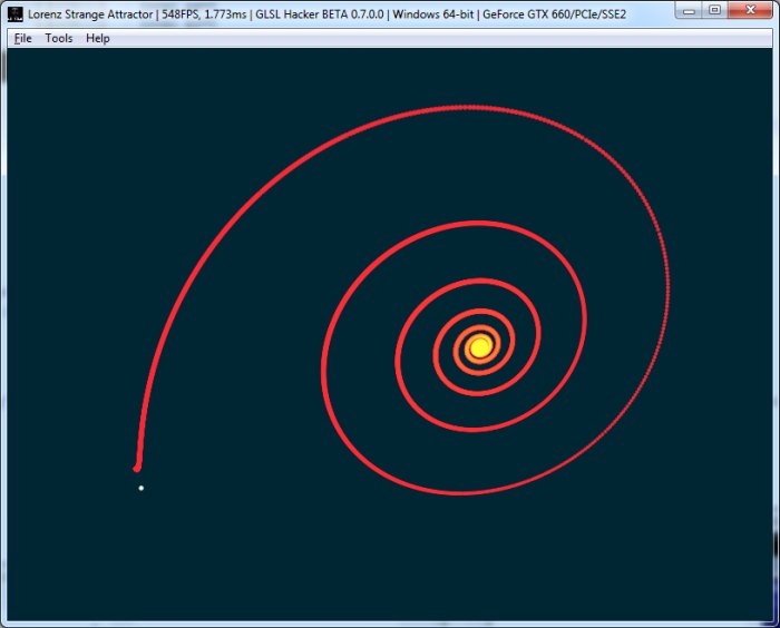
Lorenz attractor for S=2, R=28 and B=8/3
Lorenz attractor for S=10, R=60 and B=8/3
Lorenz attractor for S=10, R=20 and B=8/3
Lorenz attractor for S=12, R=30 and B=2
Lorenz attractor for S=10, R=30 and B=4.5
Adapted from this article (in french):
– Rendu de l’Attracteur de Lorenz @ 3DFR
References:
– Butterfly effect (wikipedia)
– Lorenz attractor (princeton.edu)
– The Lorenz Attractor in 3D
– Lorenz Attractor (wolfram.com)
– The Lorenz attractor (AKA the Lorenz butterfly)
– Build a Lorenz Attractor in an analog electronic circuit